Vivarium interface basics

Overview

This notebook introduces the Vivarium interface protocol by working through a simple, qualitative example of transcription/translation, and iterating on model design to add more complexity.

Note: The included examples often skirt best coding practice in favor of simplicity. See Vivarium templates on github for better starting examples: https://github.com/vivarium-collective/vivarium-template

#uncomment to install vivarium-core
#!pip install vivarium-core

# Imports and Notebook Utilities
import os
import copy
import pylab as plt
import numpy as np
from scipy import constants
import matplotlib.pyplot as plt
import matplotlib

# Process, Deriver, and Composer base classes
from vivarium.core.process import Process, Deriver
from vivarium.core.composer import Composer
from vivarium.core.registry import process_registry

# other vivarium imports
from vivarium.core.engine import Engine, pp
from vivarium.library.units import units

# plotting functions
from vivarium.plots.simulation_output import (
    plot_simulation_output, plot_variables)
from vivarium.plots.simulation_output import _save_fig_to_dir as save_fig_to_dir
from vivarium.plots.agents_multigen import plot_agents_multigen
from vivarium.plots.topology import plot_topology

# supress warnings in notebook
import warnings
warnings.filterwarnings('ignore')

AVOGADRO = constants.N_A * 1 / units.mol


# helper functions for composition
def process_in_experiment(
    process, settings, initial_state):
    composite = process.generate()
    return Engine(
        composite=composite,
        initial_state=initial_state,
        **settings)

def composite_in_experiment(
    composite, settings, initial_state):
    return Engine(
        composite=composite,
        initial_state=initial_state,
        **settings)

store_cmap = matplotlib.cm.get_cmap('Dark2')
dna_color = matplotlib.colors.to_rgba(store_cmap(0))
rna_color = matplotlib.colors.to_rgba(store_cmap(1))
protein_color = matplotlib.colors.to_rgba(store_cmap(2))
global_color = matplotlib.colors.to_rgba(store_cmap(7))
store_colors = {
    'DNA': dna_color,
    'DNA\n(counts)': dna_color,
    'DNA\n(mg/mL)': dna_color,
    'mRNA': rna_color,
    'mRNA\n(counts)': rna_color,
    'mRNA\n(mg/mL)': rna_color,
    'Protein': protein_color,
    'Protein\n(mg/mL)': protein_color,
    'global': global_color}

# plotting configurations
topology_plot_config = {
    'settings': {
        'coordinates': {
            'Tl': (-1,0),
            'Tx': (-1,-1),
            'Protein': (1,0),
            'mRNA': (1,-1),
            'DNA': (1,-2),
        },
        'node_distance': 3.0,
        'process_color': 'k',
        'store_colors': store_colors,
        'dashed_edges': True,
        'graph_format': 'vertical',
        'color_edges': False},
    'out_dir': 'out/'}

plot_var_config = {
    'row_height': 2,
    'row_padding': 0.2,
    'column_width': 10,
    'out_dir': 'out'}

Make a Process: minimal transcription

Transcription is the biological process by which RNA is synthesized from a DNA template. Here, we define a model with a single mRNA species, \(C\), transcribed from a single gene, \(G\), at transcription rate \(k_{tsc}\). RNA also degrades at rate \(k_{deg}\).

This can written as the difference equation \(\Delta RNA_{C} = (k_{tsc}[Gene_{G}] - k_{deg}[RNA_{C}]) \Delta t\)

Vivarium’s basic elements

Processes can implement any kind of dynamical model - dynamic flux balance analysis, differential equation, stochastic process, Boolean logic, etc.

Stores are databases of state variables read by the Processes, with methods for applying each Processes’ updates.

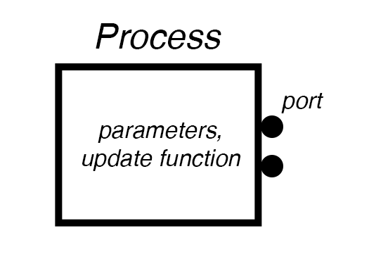
Process interface protocol

If standard modeling formats are an “HTML” for systems biology, we need an “interface protocol” such as TCP/IP serves for the internet – a protocol for connecting separate systems into a complex and open-ended network that anyone can contribute to.

Making a dynamical model into a Vivarium Process requires the following protocol: 1. A constructor that accepts parameters and configures the model. 2. A ports_schema that declares the ports and their schema. 3. A next_update that runs the model and returns an update.

Constructor

• default parameters are used in absense of an other provided parameters.

• The constructor’s parameters arguments overrides the default parameters.

class Tx(Process):

    defaults = {
        'ktsc': 1e-2,
        'kdeg': 1e-3}

    def __init__(self, parameters=None):
        super().__init__(parameters)

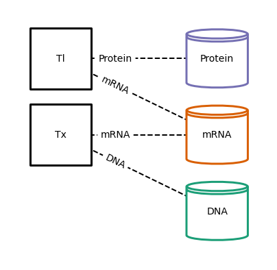
Ports Schema

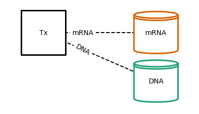
• Ports are the connections by which Process are wired to Stores.

• ports_schema declares the ports, the variables that go through them, and how those variables operate.

• Here, Tx declares a port for mRNA with variable C, and a port for DNA with variable G.

def ports_schema(self):
    return {
        'mRNA': {
            'C': {
                '_default': 0.0,
                '_updater': 'accumulate',
                '_divider': 'set',
                '_properties': {
                    'mw': 111.1 units.g / units.mol}},
        'DNA': {
            'G': {
                '_default': 1.0}}

Advanced ports_schema

• dictionary comprehensions are useful for declaring schema for configured variables.

def ports_schema(self):
    molecule_schema = {
        '_default': 0.0,
        '_emit': True}

    return {
        'molecules': {
            mol_id: molecule_schema
            for mol_id in self.parameters['molecules']}}

Advanced ports_schema

• Use the glob '*' schema to declare expected sub-store structure, and view all child values of the store:

def ports_schema(self):
    schema = {
        'port1': {
            '*': {
                '_default': 1.0
            }
        }
    }

Advanced ports_schema

• Use the glob '**' schema to connect to an entire sub-branch, including child nodes, grandchild nodes, etc:

def ports_schema(self):
    schema = {
        'port1': {
            '*': {
                '_default': 1.0
            }
        }
    }

Advanced ports_schema

• Schema methods can also be declared by passing in functions.

• The asymmetric_division divider makes molecules in the ‘front’ go to one daughter cell upon division, and those in the ‘back’ go to the other daughter.

def asymmetric_division(value, topology):
    if 'front' in topology:
        return [value, 0.0]
    elif 'back' in topology:
        return [0.0, value]

def ports_schema(self):
    return {
        'front': {
            'molecule': {
                '_divider': {
                    'divider': asymmetric_division,
                    'topology': {'front': ('molecule',)},
                }}},
        'back': {
            'molecule': {
                '_divider': {
                    'divider': asymmetric_division,
                    'topology': {'back': ('molecule',)},
                }}}}

Initial State

• Each Process MAY provide an initial_state method. This can be retrieved, reconfigured, and passed into a simulation.

• If left empty, a simulation initializes at the '_default' values.

def initial_state(self, config):
    return {
        'DNA': {'G': 1.0},
        'mRNA': {'C': 0.0}}

Update Method

• Retrieve the state variables through the ports.

• Run the model for the timestep’s duration.

• Return an update to the state variable through the ports.

def next_update(self, states, timestep):

    # Retrieve
    G = states['DNA']['G']
    C = states['mRNA']['C']

    # Run
    dC = (self.ktsc * G - self.kdeg * C) * timestep

    # Return
    return {
        'mRNA': {
            'C': dC}}

Tx: a deterministic transcription process

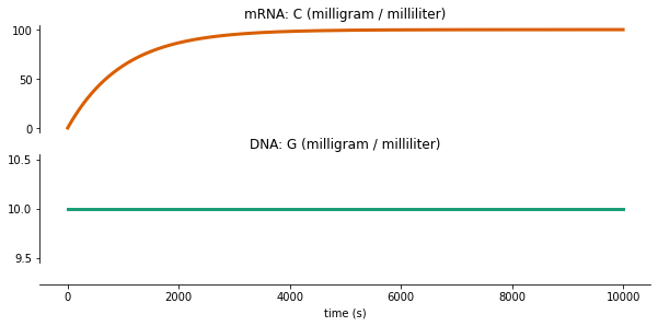
According to BioNumbers, the concentration of DNA in an E. coli cell is on the order of 11-18 mg/mL. The concentration of RNA is 75-120 mg/ml.

class Tx(Process):

    defaults = {
        'ktsc': 1e-2,
        'kdeg': 1e-3}

    def __init__(self, parameters=None):
        super().__init__(parameters)

    def ports_schema(self):
        return {
            'DNA': {
                'G': {
                    '_default': 10 * units.mg / units.mL,
                    '_updater': 'accumulate',
                    '_emit': True}},
            'mRNA': {
                'C': {
                    '_default': 100 * units.mg / units.mL,
                    '_updater': 'accumulate',
                    '_emit': True}}}

    def next_update(self, timestep, states):
        G = states['DNA']['G']
        C = states['mRNA']['C']
        dC = (self.parameters['ktsc'] * G - self.parameters['kdeg'] * C) * timestep
        return {
            'mRNA': {
                'C': dC}}

plot Tx topology

fig = plot_topology(Tx(), filename='tx_topology.pdf', **topology_plot_config)

Writing out/tx_topology.pdf

run Tx

# tsc configuration
tx_config = {'time_step': 10}
tx_sim_settings = {
    'experiment_id': 'TX'}
tx_initial_state = {
    'mRNA': {'C': 0.0 * units.mg/units.mL}}
tx_plot_config = {
    'variables': [
        {
            'variable': ('mRNA', ('C', 'milligram / milliliter')),
            'color': store_colors['mRNA']
        },
        {
            'variable': ('DNA', ('G', 'milligram / milliliter')),
            'color': store_colors['DNA']
        }],
    'filename': 'tx_output.pdf',
    **plot_var_config}

# initialize
tx_process = Tx(tx_config)

# make the experiment
tx_exp = process_in_experiment(
    tx_process, tx_sim_settings, tx_initial_state)

# run
tx_exp.update(10000)

# retrieve the data as a timeseries
tx_output = tx_exp.emitter.get_timeseries()

# plot
fig = plot_variables(tx_output,  **tx_plot_config)

Simulation ID: TX
Created: 05/18/2022 at 09:43:24
Completed in 0.283171 seconds
Writing out/tx_output.pdf

Tl: a deterministic translation process

Translation is the biological process by which protein is synthesized with an mRNA template. Here, we define a model with a single protein species, \(Protein_{X}\), transcribed from a single gene, \(RNA_{C}\), at translation rate \(k_{trl}\). Protein also degrades at rate \(k_{deg}\).

This can be represented by a chemical reaction network with the form: * $RNA_{C} \xrightarrow[]{k_{trl}} RNA_{C} + Protein_{X} $ * \(Protein_{X} \xrightarrow[]{k_{deg}} \emptyset\)

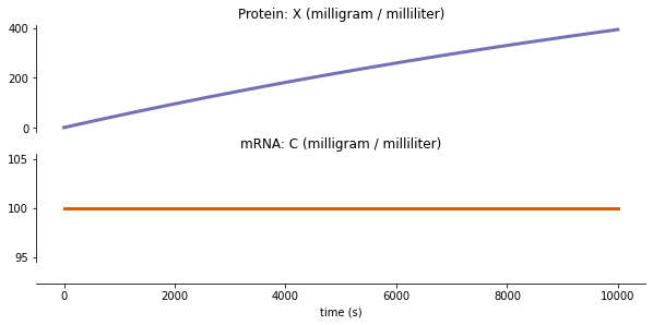
According to BioNumbers, the concentration of RNA in an E. coli cell is on the order of 75-120 mg/ml. The concentration of protein is 200-320 mg/ml.

class Tl(Process):

    defaults = {
        'ktrl': 5e-4,
        'kdeg': 5e-5}

    def ports_schema(self):
        return {
            'mRNA': {
                'C': {
                    '_default': 100 * units.mg / units.mL,
                    '_divider': 'split',
                    '_emit': True}},
            'Protein': {
                'X': {
                    '_default': 200 * units.mg / units.mL,
                    '_divider': 'split',
                    '_emit': True}}}

    def next_update(self, timestep, states):
        C = states['mRNA']['C']
        X = states['Protein']['X']
        dX = (self.parameters['ktrl'] * C - self.parameters['kdeg'] * X) * timestep
        return {
            'Protein': {
                'X': dX}}

run Tl

# trl configuration
tl_config = {'time_step': 10}
tl_sim_settings = {'experiment_id': 'TL'}
tl_initial_state = {
    'Protein': {'X': 0.0 * units.mg / units.mL}}
tl_plot_config = {
    'variables': [
        {
            'variable': ('Protein', ('X', 'milligram / milliliter')),
            'color': store_colors['Protein']
        },
        {
            'variable': ('mRNA', ('C', 'milligram / milliliter')),
            'color': store_colors['mRNA']
        },
        ],
    'filename': 'tl_output.pdf',
    **plot_var_config}

# initialize
tl_process = Tl(tl_config)

# make the experiment
tl_exp = process_in_experiment(
    tl_process, tl_sim_settings, tl_initial_state)

# run
tl_exp.update(10000)

# retrieve the data as a timeseries
tl_output = tl_exp.emitter.get_timeseries()

# plot
fig = plot_variables(tl_output,  **tl_plot_config)

Simulation ID: TL
Created: 05/18/2022 at 09:43:26
Completed in 0.297745 seconds
Writing out/tl_output.pdf

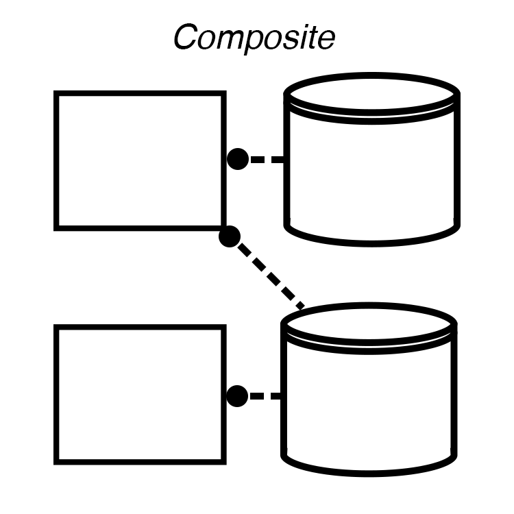
Make a Composite

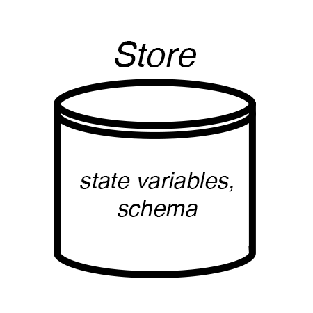
A Composite is a set of Processes and Stores. Vivarium constructs the Stores from the Processes’s port_schema methods and wires them up as instructed by a Topology. The only communication between Processes is through variables in shared Stores.

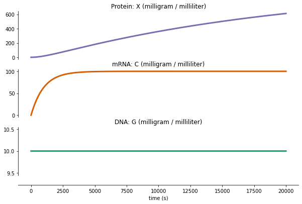
TxTl: a transcription/translation composite

We demonstrate composition by combining the Tx and Tl processes.

Composition protocol

Composers, which combine processes into composites are implemented with the protocol: 1. A constructor that accepts configuration data, which can override the consituent Processes’ default parameters. 1. A generate_processes method that constructs the Processes, passing model parameters as needed. 2. A generate_topology method that returns the Topology definition which tells Vivarium how to wire up the Processes to Stores.

composite constructor

class TxTl(Composer):

    defaults = {
        'Tx': {
            'ktsc': 1e-2},
        'Tl': {
            'ktrl': 1e-3}}

    def __init__(self, config=None):
        super().__init__(config)

generate topology

• Here, generate_topology() returns the Topology definition that wires these Processes together with 3 Stores, one of them shared.

def generate_topology(self, config):
    return {
        'Tx': {
            'DNA': ('DNA',),     # connect TSC's 'DNA' Port to a 'DNA' Store
            'mRNA': ('mRNA',)},  # connect TSC's 'mRNA' Port to a 'mRNA' Store
        'Tl': {
            'mRNA': ('mRNA',),   # connect TRL's 'mRNA' Port to the same 'mRNA' Store
            'Protein': ('Protein',)}}

advanced generate topology

• embedding in a hierarchy: to connect to sub-stores in a hierarchy, declare the path through each substore, as done to ‘lipids’.

  • To connect to supra-stores use '..' for each level up, as done to 'external'.

• splitting ports: One port can connect to multiple stores by specifying the path for each variable, as is done to 'transport'.

  • This can be used to re-map variable names, for integration of different models.

def generate_topology(config):
    return {
        'process_1': {
            'lipids': ('organelle', 'membrane', 'lipid'),
            'external': ('..', 'environment'),
            'transport': {
                'glucose_external': ('external', 'glucose'),
                'glucose_internal': ('internal', 'glucose'),
            }
        }}

TxTl Composer

class TxTl(Composer):

    defaults = {
        'Tx': {'time_step': 10},
        'Tl': {'time_step': 10}}

    def generate_processes(self, config):
        return {
            'Tx': Tx(config['Tx']),
            'Tl': Tl(config['Tl'])}

    def generate_topology(self, config):
        return {
            'Tx': {
                'DNA': ('DNA',),
                'mRNA': ('mRNA',)},
            'Tl': {
                'mRNA': ('mRNA',),
                'Protein': ('Protein',)}}

plot TxTl topology

txtl_topology_plot_config = copy.deepcopy(topology_plot_config)
txtl_topology_plot_config['settings']['node_distance'] = 2
fig = plot_topology(TxTl(), filename='txtl_topology.pdf', **topology_plot_config)

Writing out/txtl_topology.pdf

run TxTl

# tsc_trl configuration
txtl_config = {}
txtl_exp_settings = {'experiment_id': 'TXTL'}
txtl_plot_config = {
    'variables':[
        {
            'variable': ('Protein', ('X', 'milligram / milliliter')),
            'color': store_colors['Protein']
        },
        {
            'variable': ('mRNA', ('C', 'milligram / milliliter')),
            'color': store_colors['mRNA']
        },
        {
            'variable': ('DNA', ('G', 'milligram / milliliter')),
            'color': store_colors['DNA']
        },
    ],
    'filename': 'txtl_output.pdf',
    **plot_var_config}
tl_initial_state = {
    'mRNA': {'C': 0.0 * units.mg / units.mL},
    'Protein': {'X': 0.0 * units.mg / units.mL}}

# construct TxTl
txtl_composite = TxTl(txtl_config).generate()

# make the experiment
txtl_experiment = composite_in_experiment(
    txtl_composite, txtl_exp_settings, tl_initial_state)

# run it and retrieve the data that was emitted to the simulation log
txtl_experiment.update(20000)
txtl_output = txtl_experiment.emitter.get_timeseries()

# plot the output
fig = plot_variables(txtl_output, **txtl_plot_config)

Simulation ID: TXTL
Created: 05/18/2022 at 09:43:27
Completed in 0.862072 seconds
Writing out/txtl_output.pdf

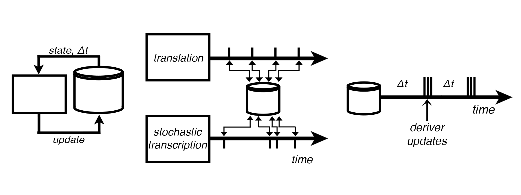
Adding Complexity

Process modularity allows modelers to iterate on model design by swapping out different models. We demonstrated this by replacing the deterministic Transcription Process with a Stochastic Transcription Process.

Stochastic transcription requires variable timesteps, which Vivarium accomodates with multi-timestepping.

StochasticTx: a stochastic transcription process

This process uses the Gillespie algorithm in its next_update() method.

stoch_exp_settings = {
    'settings': {
        'experiment_id': 'stochastic_txtl'},
    'initial_state': {
            'DNA\n(counts)': {
                'G': 1.0
            },
            'mRNA\n(counts)': {
                'C': 0.0
            },
            'Protein\n(mg/mL)': {
                'X': 0.0 * units.mg / units.mL
            }}}


stoch_plot_config = {
    'variables':[
        {
            'variable': ('Protein\n(mg/mL)', ('X', 'milligram / milliliter')),
            'color': store_colors['Protein'],
            'display': 'Protein: X (mg/mL)'},
        {
            'variable': ('mRNA\n(mg/mL)', ('C', 'milligram / milliliter')),
            'color': store_colors['mRNA'],
            'display': 'mRNA: C (mg/mL)'},
        {
            'variable': ('DNA\n(counts)', 'G'),
            'color': store_colors['DNA'],
            'display': 'DNA: G (counts)'},
    ],
    'filename': 'stochastic_txtl_output.pdf',
    **plot_var_config}

class StochasticTx(Process):

    defaults = {
        'ktsc': 1e0,
        'kdeg': 1e-3}

    def __init__(self, parameters=None):
        super().__init__(parameters)
        self.ktsc = self.parameters['ktsc']
        self.kdeg = self.parameters['kdeg']
        self.stoichiometry = np.array([[0, 1], [0, -1]])
        self.time_left = None
        self.event = None

        # initialize the next timestep
        initial_state = self.initial_state()
        self.calculate_timestep(initial_state)

    def initial_state(self, config=None):
        return {
            'DNA': {
                'G': 1.0
            },
            'mRNA': {
                'C': 1.0
            }
        }

    def ports_schema(self):
        return {
            'DNA': {
                'G': {
                    '_default': 1.0,
                    '_emit': True}},
            'mRNA': {
                'C': {
                    '_default': 1.0,
                    '_emit': True}}}

    def calculate_timestep(self, states):
        # retrieve the state values
        g = states['DNA']['G']
        c = states['mRNA']['C']

        array_state = np.array([g, c])

        # Calculate propensities
        propensities = [
            self.ktsc * array_state[0], self.kdeg * array_state[1]]
        prop_sum = sum(propensities)

        # The wait time is distributed exponentially
        self.calculated_timestep = np.random.exponential(scale=prop_sum)
        return self.calculated_timestep

    def next_reaction(self, x):
        """get the next reaction and return a new state"""

        propensities = [self.ktsc * x[0], self.kdeg * x[1]]
        prop_sum = sum(propensities)

        # Choose the next reaction
        r_rxn = np.random.uniform()
        i = 0
        for i, _ in enumerate(propensities):
            if r_rxn < propensities[i] / prop_sum:
                # This means propensity i fires
                break
        x += self.stoichiometry[i]
        return x

    def next_update(self, timestep, states):

        if self.time_left is not None:
            if timestep >= self.time_left:
                event = self.event
                self.event = None
                self.time_left = None
                return event

            self.time_left -= timestep
            return {}

        # retrieve the state values, put them in array
        g = states['DNA']['G']
        c = states['mRNA']['C']
        array_state = np.array([g, c])

        # calculate the next reaction
        new_state = self.next_reaction(array_state)

        # get delta mRNA
        c1 = new_state[1]
        d_c = c1 - c

        update = {
            'mRNA': {
                'C': d_c}}

        if self.calculated_timestep > timestep:
            # didn't get all of our time, store the event for later
            self.time_left = self.calculated_timestep - timestep
            self.event = update
            return {}

        # return an update
        return {
            'mRNA': {
                'C': d_c}}

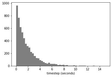
plot variable timesteps

stoch_tx_process = StochasticTx(tx_config)
stoch_tx_exp = process_in_experiment(stoch_tx_process, **stoch_exp_settings)
stoch_tx_exp.update(10000)
stoch_tx_output = stoch_tx_exp.emitter.get_timeseries()



# calculate the timesteps
times = stoch_tx_output['time']
timesteps = []
for x, y in zip(times[0::], times[1::]):
#     if y-x != 1.0:
        timesteps.append(y-x)

fig = plt.hist(timesteps, 50, color='tab:gray')
plt.xlabel('timestep (seconds)')
plt.savefig('out/stochastic_timesteps.pdf')

Simulation ID: stochastic_txtl
Created: 05/18/2022 at 09:43:29
Completed in 0.473557 seconds

Auxiliary Processes

• Connecting different Processes may require addition ‘helper’ Processes to make conversions and adapt their unique requirements different values.

• Derivers are a subclass of Process that runs after the other dynamic Processes and derives some states from others.

A concentration deriver convert the counts of the stochastic process to concentrations. This is available in the process_registry

concentrations_deriver = process_registry.access('concentrations_deriver')

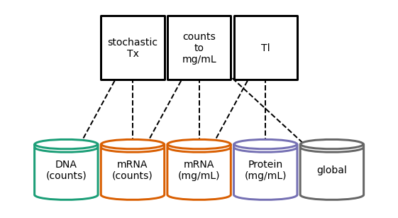
Combining stochastic Tx with deterministic Tl

# configuration data
mw_config = {'C': 1e8 * units.g / units.mol}

class StochasticTxTl(Composer):
    defaults = {
        'stochastic_Tx': {},
        'Tl': {'time_step': 1},
        'concs': {
            'molecular_weights': mw_config}}

    def generate_processes(self, config):
        counts_to_concentration = process_registry.access('counts_to_concentration')
        return {
            'stochastic\nTx': StochasticTx(config['stochastic_Tx']),
            'Tl': Tl(config['Tl']),
            'counts\nto\nmg/mL': counts_to_concentration(config['concs'])}

    def generate_topology(self, config):
        return {
            'stochastic\nTx': {
                'DNA': ('DNA\n(counts)',),
                'mRNA': ('mRNA\n(counts)',)
            },
            'Tl': {
                'mRNA': ('mRNA\n(mg/mL)',),
                'Protein': ('Protein\n(mg/mL)',)
            },
            'counts\nto\nmg/mL': {
                'global': ('global',),
                'input': ('mRNA\n(counts)',),
                'output': ('mRNA\n(mg/mL)',)
            }}

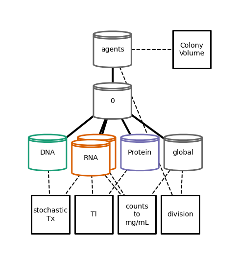
plot StochasticTxTl topology

# plot topology after merge
stochastic_topology_plot_config = copy.deepcopy(topology_plot_config)
stochastic_topology_plot_config['settings']['graph_format'] = 'horizontal'
stochastic_topology_plot_config['settings']['coordinates'] = {
    'stochastic\nTx': (2, 1),
    'counts\nto\nmg/mL': (3, 1),
    'Tl': (4, 1),
    'DNA\n(counts)': (1,-1),
    'mRNA\n(counts)': (2,-1),
    'mRNA\n(mg/mL)': (3,-1),
    'Protein\n(mg/mL)': (4,-1)}
stochastic_topology_plot_config['settings']['dashed_edges'] = True
stochastic_topology_plot_config['settings']['show_ports'] = False
stochastic_topology_plot_config['settings']['node_distance'] = 2.2


stochastic_txtl = StochasticTxTl()
fig = plot_topology(
    stochastic_txtl,
    filename='stochastic_txtl_topology.pdf',
    **stochastic_topology_plot_config)

Writing out/stochastic_txtl_topology.pdf

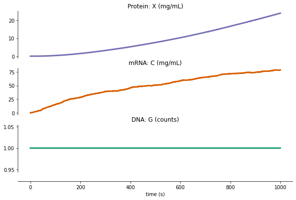
run StochasticTxTl

# make the experiment
stoch_experiment = composite_in_experiment(stochastic_txtl.generate(), **stoch_exp_settings)

# simulate and retrieve the data
stoch_experiment.update(1000)
stochastic_txtl_output = stoch_experiment.emitter.get_timeseries()

# plot output
fig = plot_variables(stochastic_txtl_output, **stoch_plot_config)

Simulation ID: stochastic_txtl
Created: 05/18/2022 at 09:43:30
Completed in 0.983180 seconds
Writing out/stochastic_txtl_output.pdf

Growth and Division

We here extend the Transcription/Translation model with division. This require many instances of the processes to run simultaneously in a single simulation. To support such phenomena, Vivarium adopts an agent-based modeling bigraphical formalism, with embedded compartments that can spawn new compartments during runtime.

Hierarchical Embedding

To support this requirement, Processes can be embedded in a hierarchical representation of embedded compartments. Vivarium uses a bigraph formalism – a graph with embeddable nodes that can be placed within other nodes.

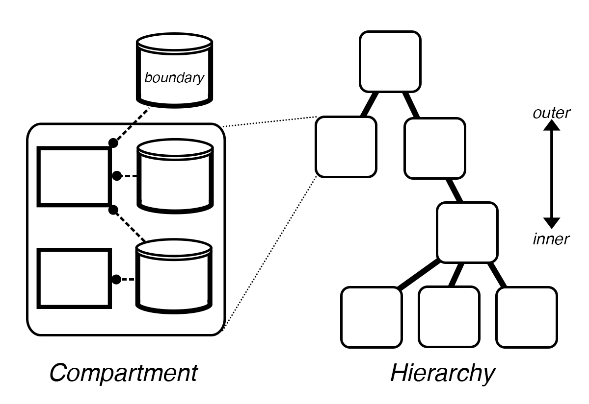
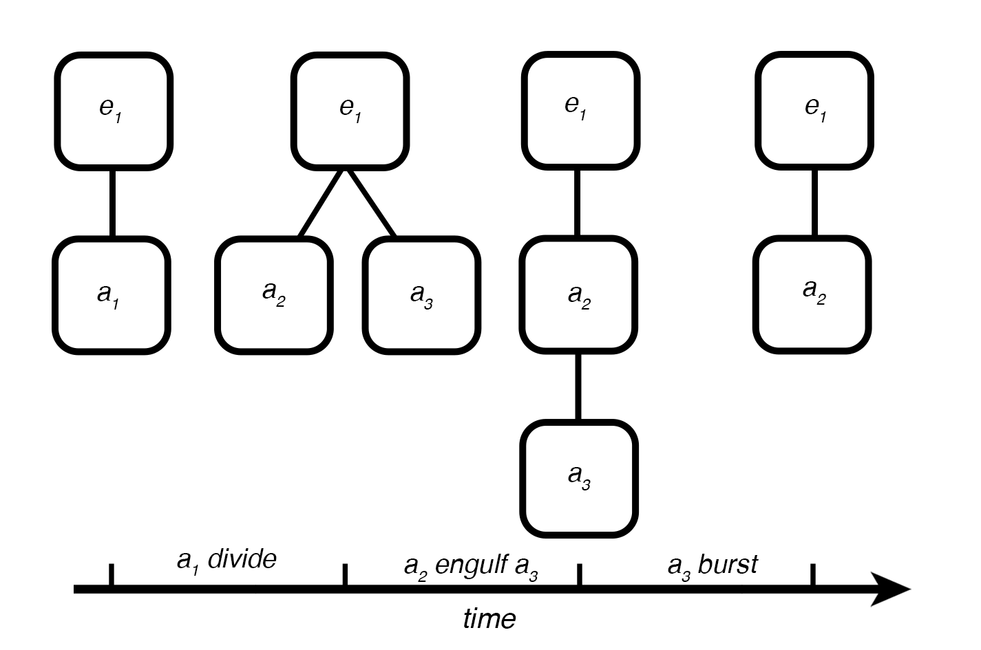
Hierarchy updates

The structure of a hierarchy has its own type of constructive dynamics with formation/destruction, merging/division, engulfing/expelling of compartments

# add imported division processes
from vivarium.processes.divide_condition import DivideCondition
from vivarium.processes.meta_division import MetaDivision
from vivarium.processes.growth_rate import GrowthRate

TIMESTEP = 10


class TxTlDivision(Composer):
    defaults = {
        'stochastic_Tx': {'time_step': TIMESTEP},
        'Tl': {'time_step': TIMESTEP},
        'concs': {
            'molecular_weights': mw_config},
        'growth': {
            'time_step': 1,
            'default_growth_rate': 0.0005,
            'default_growth_noise': 0.001,
            'variables': ['volume']},
        'agent_id': np.random.randint(0, 100),
        'divide_condition': {
            'threshold': 2.5 * units.fL},
        'agents_path': ('..', '..', 'agents',),
        'daughter_path': tuple(),
        '_schema': {
            'concs': {
                'input': {'C': {'_divider': 'binomial'}},
                'output': {'C': {'_divider': 'set'}},
            }
        }
    }

    def generate_processes(self, config):
        counts_to_concentration = process_registry.access('counts_to_concentration')
        division_config = dict(
            daughter_path=config['daughter_path'],
            agent_id=config['agent_id'],
            composer=self)

        return {
            'stochastic_Tx': StochasticTx(config['stochastic_Tx']),
            'Tl': Tl(config['Tl']),
            'concs': counts_to_concentration(config['concs']),
            'growth': GrowthRate(config['growth']),
            'divide_condition': DivideCondition(config['divide_condition']),
            'division': MetaDivision(division_config),
        }

    def generate_topology(self, config):
        return {
            'stochastic_Tx': {
                'DNA': ('DNA',),
                'mRNA': ('RNA_counts',)
            },
            'Tl': {
                'mRNA': ('RNA',),
                'Protein': ('Protein',)
            },
            'concs': {
                'global': ('global',),
                'input': ('RNA_counts',),
                'output': ('RNA',)
            },
            'growth': {
                'variables': ('global',),
                'rates': ('rates',)
            },
            'divide_condition': {
                'variable': ('global', 'volume',),
                'divide': ('global', 'divide',)},
            'division': {
                'global': ('global',),
                'agents': config['agents_path']}
        }

Colony-level processes

from vivarium.library.units import Quantity

def calculate_volume(value, path, node):
    if isinstance(node.value, Quantity) and node.units == units.fL:
        return value + node.value
    else:
        return value

class ColonyVolume(Deriver):
    defaults = {
        'colony_path': ('..', '..', 'agents')}
    def ports_schema(self):
        return {
            'colony': {
                'volume': {
                    '_default': 1.0 * units.fL,
                    '_updater': 'set',
                    '_emit': True}}}
    def next_update(self, timestep, states):
        return {
            'colony': {
                'volume': {
                    '_reduce': {
                        'reducer': calculate_volume,
                        'from': self.parameters['colony_path'],
                        'initial': 0.0 * units.fL}}}}

# configure hierarchy
# agent config
agent_id = '0'
agent_config = {'agent_id': agent_id}

# environment config
env_config = {}

# initial state
hierarchy_initial_state = {
    'agents': {
        agent_id: {
            'global': {'volume': 1.2 * units.fL},
            'DNA': {'G': 1},
            'RNA': {'C': 5 * units.mg / units.mL},
            'Protein': {'X': 50 * units.mg / units.mL}}}}

# experiment settings
exp_settings = {
    'experiment_id': 'hierarchy_experiment',
    'initial_state': hierarchy_initial_state,
    'emit_step': 100.0}

# plot config
hierarchy_plot_settings = {
    'include_paths': [
        ('RNA_counts', 'C'),
        ('RNA', 'C'),
        ('DNA', 'G'),
        ('Protein', 'X'),
    ],
    'store_order': ('Protein', 'RNA_counts', 'DNA', 'RNA'),
    'titles_map': {
        ('Protein', 'X',): 'Protein',
        ('RNA_counts', 'C'): 'RNA',
        ('DNA', 'G',): 'DNA',
        'RNA': 'RNA',
    },
    'column_width': 6,
    'row_height': 1.0,
    'stack_column': True,
    'tick_label_size': 10,
    'linewidth': 1,
    'title_size': 10}

colony_plot_config = {
    'variables': [('global', ('volume', 'femtoliter'))],
    'filename': 'colony_growth.pdf',
    **plot_var_config}


# hierarchy topology plot
agent_0_string = 'agents\n0'
agent_1_string = 'agents\n00'
agent_2_string = 'agents\n01'
row_1 = 0
row_2 = -1
row_3 = -2
row_4 = -3
node_space = 0.75
vertical_space=0.9
bump = 0.1
process_column = -0.2
agent_row = -3.2
agent_column = bump/2 #0.5

hierarchy_topology_plot_config = {
    'settings': {
        'graph_format': 'hierarchy',
        'node_size': 6000,
        'process_color': 'k',
        'store_color': global_color,
        'store_colors': {
            f'{agent_0_string}\nDNA': dna_color,
            f'{agent_0_string}\nRNA': rna_color,
            f'{agent_0_string}\nRNA_counts': rna_color,
            f'{agent_0_string}\nProtein': protein_color,
        },
        'dashed_edges': True,
        'show_ports': False,
        'coordinates': {
            # Processes
            'ColonyVolume': (2.5, 0),
            'agents\n0\nstochastic_Tx': (agent_column, agent_row*vertical_space),
            'agents\n0\nTl': (agent_column+node_space, agent_row*vertical_space),
            'agents\n0\nconcs': (agent_column+2*node_space, agent_row*vertical_space),
            'agents\n0\ndivision': (agent_column+3*node_space, agent_row*vertical_space),
            # Stores
            'agents': (1.5*node_space, row_1*vertical_space),
            'agents\n0': (1.5*node_space, row_2*vertical_space),
            'agents\n0\nagents': (1.5*node_space, row_1*vertical_space),
            'agents\n0\nDNA': (0, row_3*vertical_space),
            'agents\n0\nRNA_counts': (node_space+bump, row_3*vertical_space),
            'agents\n0\nRNA': (node_space, (row_3-bump)*vertical_space),
            'agents\n0\nProtein': (2*node_space+bump, row_3*vertical_space),
            'agents\n0\nglobal': (3*node_space+bump, row_3*vertical_space),
        },
        'node_labels': {
            # Processes
            'ColonyVolume': 'Colony\nVolume',
            'agents\n0\nstochastic_Tx': 'stochastic\nTx',
            'agents\n0\nTl': 'Tl',
            'agents\n0\nconcs': 'counts\nto\nmg/mL',
            'agents\n0\ngrowth': 'growth',
            'agents\n0\ndivision': 'division',
            # Stores
            # third
            'agents\n0': '0',
            'agents\n0\nDNA': 'DNA',
            'agents\n0\nRNA': 'RNA',
            'agents\n0\nrates': 'rates',
            'agents\n0\nRNA_counts': '',
            'agents\n0\nglobal': 'global',
            'agents\n0\nProtein': 'Protein',
            # fourth
            'agents\n0\nrates\ngrowth_rate': 'growth_rate',
            'agents\n0\nrates\ngrowth_noise': 'growth_noise',
        },
        'remove_nodes': [
            'agents\n0\nrates\ngrowth_rate',
            'agents\n0\nrates\ngrowth_noise',
            'agents\n0\nrates',
            'agents\n0\ngrowth',
            'agents\n0\ndivide_condition',
            'agents\n0\nglobal\ndivide',
            'agents\n0\nglobal\nvolume',
        ]
    },
    'out_dir': 'out/'
}

# topology plot config for after division
agent_2_dist = 3.5
hierarchy_topology_plot_config2 = copy.deepcopy(hierarchy_topology_plot_config)

# redo coordinates, labels, store_colors, and removal
hierarchy_topology_plot_config2['settings']['node_distance'] = 2.5
hierarchy_topology_plot_config2['settings']['coordinates'] = {}
hierarchy_topology_plot_config2['settings']['node_labels'] = {}
hierarchy_topology_plot_config2['settings']['store_colors'] = {}
# hierarchy_topology_plot_config2['settings']['remove_nodes'] = []
for node_id, coord in hierarchy_topology_plot_config['settings']['coordinates'].items():
    if agent_0_string in node_id:
        new_id1 = node_id.replace(agent_0_string, agent_1_string)
        new_id2 = node_id.replace(agent_0_string, agent_2_string)
        hierarchy_topology_plot_config2['settings']['coordinates'][new_id1] = coord
        hierarchy_topology_plot_config2['settings']['coordinates'][new_id2] = (coord[0]+agent_2_dist, coord[1])
    else:
        hierarchy_topology_plot_config2['settings']['coordinates'][node_id] = (coord[0]+agent_2_dist/2, coord[1])
hierarchy_topology_plot_config2['settings']['coordinates']['ColonyVolume'] = (5.5, 0)

for node_id, label in hierarchy_topology_plot_config['settings']['node_labels'].items():
    if agent_0_string in node_id:
        new_id1 = node_id.replace(agent_0_string, agent_1_string)
        new_id2 = node_id.replace(agent_0_string, agent_2_string)
        hierarchy_topology_plot_config2['settings']['node_labels'][new_id1] = label
        hierarchy_topology_plot_config2['settings']['node_labels'][new_id2] = label
    else:
        hierarchy_topology_plot_config2['settings']['node_labels'][node_id] = label
hierarchy_topology_plot_config2['settings']['node_labels']['agents\n00'] = '1'
hierarchy_topology_plot_config2['settings']['node_labels']['agents\n01'] = '2'

for node_id, color in hierarchy_topology_plot_config['settings']['store_colors'].items():
    if agent_0_string in node_id:
        new_id1 = node_id.replace(agent_0_string, agent_1_string)
        new_id2 = node_id.replace(agent_0_string, agent_2_string)
        hierarchy_topology_plot_config2['settings']['store_colors'][new_id1] = color
        hierarchy_topology_plot_config2['settings']['store_colors'][new_id2] = color
    else:
        hierarchy_topology_plot_config2['settings']['store_colors'][node_id] = color

for node_id in hierarchy_topology_plot_config['settings']['remove_nodes']:
    if agent_0_string in node_id:
        new_id1 = node_id.replace(agent_0_string, agent_1_string)
        new_id2 = node_id.replace(agent_0_string, agent_2_string)
        hierarchy_topology_plot_config2['settings']['remove_nodes'].extend([new_id1, new_id2])

use composite.merge to combine colony processes with agents

# make a txtl composite, embedded under an agents store
txtl_composer = TxTlDivision(agent_config)
hierarchy_composite = txtl_composer.generate(path=('agents', agent_id))

# make a colony composite, and a topology that connects its colony port to agents store
colony_composer = ColonyVolume(env_config)
colony_composite = colony_composer.generate()
colony_topology = {'ColonyVolume': {'colony': ('agents',)}}

# perform merge
hierarchy_composite.merge(composite=colony_composite, topology=colony_topology)

plot hierarchy topology with before division

fig = plot_topology(
    hierarchy_composite,
    filename='hierarchy_topology.pdf',
    **hierarchy_topology_plot_config)

Writing out/hierarchy_topology.pdf

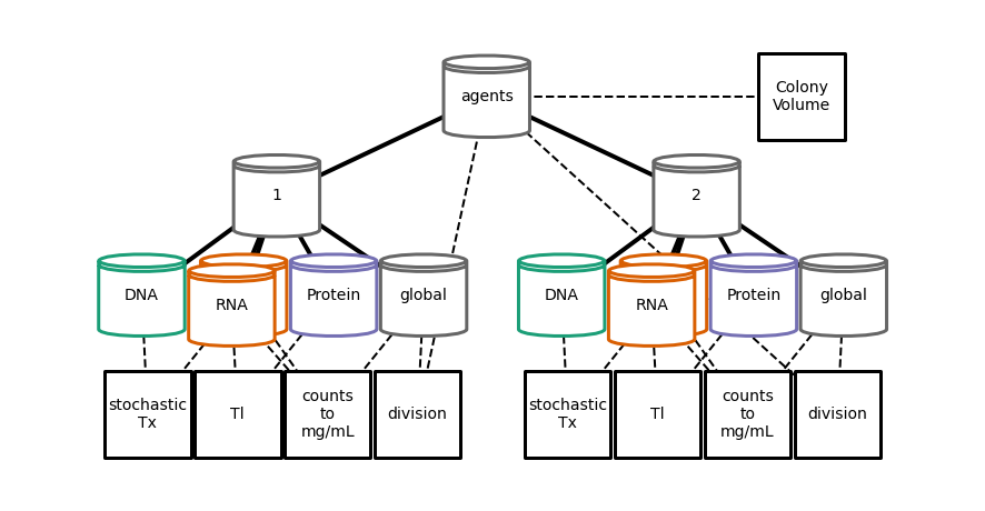
plot hierarchy topology after division

# initial state
initial_state = {
    'agents': {
        agent_id: {
            'global': {'volume': 1.2 * units.fL},
            'DNA': {'G': 1},
            'RNA': {'C': 5 * units.mg / units.mL},
            'Protein': {'X': 50 * units.mg / units.mL}}}}

# make a copy of the composite
txtl_composite1 = copy.deepcopy(hierarchy_composite)

# make the experiment
hierarchy_experiment1 = composite_in_experiment(
    composite=txtl_composite1,
    settings={},
    initial_state=initial_state)

# run the experiment long enough to divide
hierarchy_experiment1.update(2000)

Simulation ID: a7e6aa2e-d6c9-11ec-8a5b-8c85908ac627
Created: 05/18/2022 at 09:43:33
Completed in 5.25 seconds

fig = plot_topology(
    txtl_composite1,
    filename='hierarchy_topology_2.pdf',
    **hierarchy_topology_plot_config2)

Writing out/hierarchy_topology_2.pdf

run hierarchy experiment

# initial state
initial_state = {
    'agents': {
        agent_id: {
            'global': {'volume': 1.2 * units.fL},
            'DNA': {'G': 1},
            'RNA': {'C': 5 * units.mg / units.mL},
            'Protein': {'X': 50 * units.mg / units.mL}}}}

# make the experiment
hierarchy_experiment = composite_in_experiment(
    composite=hierarchy_composite,
    settings={},
    initial_state=initial_state)

# run the experiment
hierarchy_experiment.update(6000)

Simulation ID: ab2e8210-d6c9-11ec-8a5b-8c85908ac627
Created: 05/18/2022 at 09:43:39
Completed in 117.13 seconds

# retrieve the data
hierarchy_data = hierarchy_experiment.emitter.get_data_unitless()
path_ts = hierarchy_experiment.emitter.get_path_timeseries()

# add agent colors
dimgray = (0.4,0.4,0.4)
paths = list(path_ts.keys())
agent_ids = set([path[1] for path in paths if '0' in path[1]])
agent_colors = {agent_id: dimgray for agent_id in agent_ids}
hierarchy_plot_settings.update({'agent_colors': agent_colors})

# initialize the plot
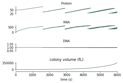
multigen_fig = plot_agents_multigen(hierarchy_data, hierarchy_plot_settings)
plt.close()

Colony-level metrics

gd_timeseries = hierarchy_experiment.emitter.get_timeseries()
colony_series = gd_timeseries['agents'][('volume', 'femtoliter')]
time_vec = gd_timeseries['time']

# get the RNA_counts axis, to replace with colony volume
allaxes = multigen_fig.get_axes()
ax = None
for axis in allaxes:
    if axis.get_title() == 'RNA \nC':
        ax = axis

# multigen_fig
ax.clear()
ax.plot(time_vec, colony_series, linewidth=1.0, color='darkslategray')
ax.set_xlim([time_vec[0], time_vec[-1]])
ax.set_title('colony volume (fL)', rotation=0)
ax.set_xlabel('time (s)')
ax.spines['bottom'].set_position(('axes', -0.2))
save_fig_to_dir(multigen_fig, 'growth_division_output.pdf')
multigen_fig

Writing out/growth_division_output.pdf